Selective inference for TransFusion Feature Selection

TransFusion in [6] is a robust transfer learning method designed to handle covariate shift between source and target domains. This example provides the post-selection inference for the TransFusion feature selection, using framework proposed in [5]. [5] Tam, N. V. K., My, C. H., & Duy, V. N. L. (2025). Post-Transfer Learning Statistical Inference in High-Dimensional Regression. arXiv preprint arXiv:2504.18212. [6] He, Z., Sun, Y., & Li, R. (2024, April). Transfusion: Covariate-shift robust transfer learning for high-dimensional regression. In International Conference on Artificial Intelligence and Statistics (pp. 703-711). PMLR.

# Author: Nguyen Vu Khai Tam & Cao Huyen My

from pythonsi import Pipeline
from pythonsi.transfer_learning_hdr import TLTransFusion
from pythonsi import Data
from pythonsi.test_statistics import TLHDRTestStatistic
import numpy as np
import matplotlib.pyplot as plt

Generate data

def generate_coef(p, s, true_beta=0.25, num_info_aux=3, num_uninfo_aux=2, gamma=0.01):
    K = num_info_aux + num_uninfo_aux
    beta_0 = np.concatenate([np.full(s, true_beta), np.zeros(p - s)])

    Beta_S = np.tile(beta_0, (K, 1)).T
    if s >= 0:
        Beta_S[0, :] -= 2 * true_beta
        for m in range(K):
            if m < num_uninfo_aux:
                Beta_S[:50, m] += np.random.normal(0, true_beta * gamma * 10, 50)
            else:
                Beta_S[:25, m] += np.random.normal(0, true_beta * gamma, 25)
    return Beta_S, beta_0


def generate_data(
    p, s, nS, nT, true_beta=0.25, num_info_aux=3, num_uninfo_aux=2, gamma=0.01
):
    K = num_info_aux + num_uninfo_aux

    Beta_S, beta_0 = generate_coef(p, s, true_beta, num_info_aux, num_uninfo_aux, gamma)
    Beta = np.column_stack([Beta_S[:, i] for i in range(K)] + [beta_0])

    X_list = []
    Y_list = []

    cov = np.eye(p)
    N_vec = [nS] * K + [nT]

    for k in range(K + 1):
        Xk = np.random.multivariate_normal(mean=np.zeros(p), cov=cov, size=N_vec[k])
        true_Yk = Xk @ Beta[:, k]
        noise = np.random.normal(0, 1, N_vec[k])
        # noise = np.random.laplace(0, 1, N_vec[k])
        # noise = skewnorm.rvs(a=10, loc=0, scale=1, size=N_vec[k])
        # noise = np.random.standard_t(df=20, size=N_vec[k])
        Yk = true_Yk + noise
        X_list.append(Xk)
        Y_list.append(Yk.reshape(-1, 1))

    XS_list = np.array(X_list[:-1])
    YS_list = np.array(Y_list[:-1]).reshape(-1, 1)
    X0 = X_list[-1]
    Y0 = Y_list[-1]
    SigmaS_list = np.array([np.eye(nS) for _ in range(K)])
    Sigma0 = np.eye(nT)

    return XS_list, YS_list, X0, Y0, SigmaS_list, Sigma0


def compute_adaptive_weights(K, nS, nT):
    ak = 8.0 * np.sqrt(nS / (K * nS + nT))
    return [ak] * K

Define hyper-parameters

p = 100
s = 5
true_beta = 1
gamma = 0.1
nS = 50
nT = 50
num_uninfo_aux = 2
num_info_aux = 3
K = num_info_aux + num_uninfo_aux
N = nS * K + nT
ak_weights = compute_adaptive_weights(K, nS, nT)
lambda_0 = np.sqrt(np.log(p) / N) * 4
lambda_tilde = np.sqrt(np.log(p) / nT) * 2

Define pipeline

def PTL_SI_TL() -> Pipeline:
    XS_list = Data()
    YS_list = Data()
    X0 = Data()
    Y0 = Data()
    SigmaS_list = Data()
    Sigma0 = Data()

    transfusion = TLTransFusion(lambda_0, lambda_tilde, ak_weights)
    active_set = transfusion.run(XS_list, YS_list, X0, Y0)
    return Pipeline(
        inputs=(XS_list, YS_list, X0, Y0, SigmaS_list, Sigma0),
        output=active_set,
        test_statistic=TLHDRTestStatistic(
            XS_list=XS_list, YS_list=YS_list, X0=X0, Y0=Y0
        ),
    )


my_pipeline = PTL_SI_TL()

Run the pipeline

XS_list, YS_list, X0, Y0, SigmaS_list, Sigma0 = generate_data(
    p, s, nS, nT, true_beta, num_info_aux, num_uninfo_aux, gamma
)
selected_features, p_values = my_pipeline(
    inputs=[XS_list, YS_list, X0, Y0], covariances=[SigmaS_list, Sigma0], verbose=True
)
print("Selected features: ", selected_features)
print("P-values: ", p_values)

Selected output: [ 0  1  2  3  4 12 14 21 22 23 27 38 43 55]
Testing feature 0
Feature 0: p-value = 0.0017418800539716894
Testing feature 1
Feature 1: p-value = 0.01893713251625795
Testing feature 2
Feature 2: p-value = 3.1372704434318166e-10
Testing feature 3
Feature 3: p-value = 0.0988403336500121
Testing feature 4
Feature 4: p-value = 0.14624944764658854
Testing feature 5
Feature 5: p-value = 0.18912361352651288
Testing feature 6
Feature 6: p-value = 0.8836702327309743
Testing feature 7
Feature 7: p-value = 0.04802244992814873
Testing feature 8
Feature 8: p-value = 0.6017183926169747
Testing feature 9
Feature 9: p-value = 0.14585800418510592
Testing feature 10
Feature 10: p-value = 0.016176601474066885
Testing feature 11
Feature 11: p-value = 0.17624726690576398
Testing feature 12
Feature 12: p-value = 0.23644058502301757
Testing feature 13
Feature 13: p-value = 0.05226088699866338
Selected features:  [ 0  1  2  3  4 12 14 21 22 23 27 38 43 55]
P-values:  [0.0017418800539716894, 0.01893713251625795, 3.1372704434318166e-10, 0.0988403336500121, 0.14624944764658854, 0.18912361352651288, 0.8836702327309743, 0.04802244992814873, 0.6017183926169747, 0.14585800418510592, 0.016176601474066885, 0.17624726690576398, 0.23644058502301757, 0.05226088699866338]

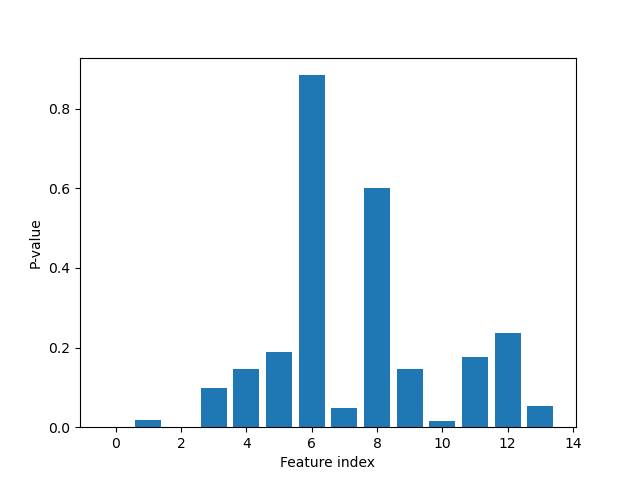
Plot p-values

plt.figure()
plt.bar(range(len(p_values)), p_values)
plt.xlabel("Feature index")
plt.ylabel("P-value")
plt.show()