SI for Sequential Feature Selection after Optimal Transport-based Domain Adaptation

This example demonstrates how to perform statistical inference for sequential feature selection (SeqFS) after applying Optimal Transport-based Domain Adaptation. The implementation follows the methodology proposed by Loc et al. (2025) [4]. [4] Loc, D. T., Loi, N. T., & Duy, V. N. L. (2025). Statistical Inference for Sequential Feature Selection after Domain Adaptation. arXiv preprint arXiv:2501.09933.

# Author: Duong Tan Loc

from pythonsi import Pipeline
from pythonsi.feature_selection import SequentialFeatureSelection
from pythonsi import Data
from pythonsi.test_statistics import SFS_DATestStatistic
from pythonsi.domain_adaptation import OptimalTransportDA
import numpy as np
import matplotlib.pyplot as plt

Define the pipeline

def SI_SeqFS_DA(k) -> Pipeline:
    xs = Data()
    ys = Data()

    xt = Data()
    yt = Data()

    OT = OptimalTransportDA()
    x_tilde, y_tilde = OT.run(xs=xs, ys=ys, xt=xt, yt=yt)

    seqfs = SequentialFeatureSelection(k, direction="forward")
    active_set = seqfs.run(x_tilde, y_tilde)
    return Pipeline(
        inputs=(xs, ys, xt, yt),
        output=active_set,
        test_statistic=SFS_DATestStatistic(xs=xs, ys=ys, xt=xt, yt=yt),
    )


my_pipeline = SI_SeqFS_DA(3)

Generate data

def gen_data(n, p, true_beta):
    x = np.random.normal(loc=0, scale=1, size=(n, p))
    true_beta = true_beta.reshape(-1, 1)

    mu = x.dot(true_beta)
    Sigma = np.identity(n)
    Y = mu + np.random.normal(loc=0, scale=1, size=(n, 1))
    return x, Y, Sigma


xs, ys, sigma_s = gen_data(150, 5, np.asarray([0, 0, 0, 0, 0]))
xt, yt, sigma_t = gen_data(25, 5, np.asarray([0, 0, 0, 0, 0]))

Run the pipeline

selected_features, p_values = my_pipeline(
    inputs=[xs, ys, xt, yt], covariances=[sigma_s, sigma_t]
)

print("Selected features: ", selected_features)
print("P-values: ", p_values)

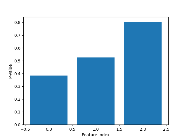
Selected features:  [3, 4, 1]
P-values:  [0.38409760959246575, 0.5261348213591066, 0.8038003268473604]

Plot the p-values

plt.figure()
plt.bar(range(len(p_values)), p_values)
plt.xlabel("Feature index")
plt.ylabel("P-value")
plt.show()